Quantum Mechanics 2

1. Wave Function

Theorem

the schrodinger equation is given by

i ℏ \frac{\partial Ψ}{\partial t} = - \frac{ℏ^{2}}{2 m} \frac{\partial^{2} Ψ}{\partial x^{2}} + V Ψ .

where the reduced planck constant is $ℏ = \frac{h}{2 π}$ and that

\int_{a}^{b} | Ψ (x, t) |^{2} d x

is the area under the graph of $| Ψ |^{2}$ which represents the probability of finding particle at point x at time t between a,b. Because this a probability we must have

\int_{- \infty}^{+ \infty} | Ψ (x, t) |^{2} d x = 1.

However we see that from the schrodinger equation above if $Ψ (x, t)$ is a solution then so must $A Ψ (x, t)$ since it is a linear PDE. Hence in order to satisfy this condition we go through a process called normalization which refers to pikcing a mulitplicative factor that makes this integral 1 as desired. If no such multiplicative factor exists than it is non-normalizable. This also includes the case of $Ψ = 0$ this does not represent particles.(zero function basically means the particle disappears at all positions and times)

Question

suppose that the wave function is normalized at some time say $t = 0$ but how do we know that this wave function will normalized as time evolves?

we may differentiate under the integral like so(since $Ψ (x, t) \to 0, x \to \pm \infty$ i.e vanishes at boundary)

\frac{d}{d t} \int_{- \infty}^{+ \infty} | Ψ (x, t) |^{2} d x = \int_{- \infty}^{+ \infty} \frac{\partial}{\partial t} | Ψ (x, t) |^{2} d x .

next see that

\frac{\partial}{\partial t} | Ψ |^{2} = \frac{\partial}{\partial t} (Ψ^{\*} Ψ) = Ψ^{\*} \frac{\partial Ψ}{\partial t} + \frac{\partial Ψ^{\*}}{\partial t} Ψ .

Now the Schrödinger equation says that

\frac{\partial Ψ}{\partial t} = \frac{i ℏ}{2 m} \frac{\partial^{2} Ψ}{\partial x^{2}} - \frac{i}{ℏ} V Ψ,

and hence also (taking the complex conjugate of above)

\frac{\partial Ψ^{\*}}{\partial t} = - \frac{i ℏ}{2 m} \frac{\partial^{2} Ψ^{\*}}{\partial x^{2}} + \frac{i}{ℏ} V Ψ^{\*},

\frac{\partial}{\partial t} | Ψ |^{2} = \frac{i ℏ}{2 m} (Ψ^{\*} \frac{\partial^{2} Ψ}{\partial x^{2}} - \frac{\partial^{2} Ψ^{\*}}{\partial x^{2}} Ψ) = \frac{\partial}{\partial x} [\frac{i ℏ}{2 m} (Ψ^{\*} \frac{\partial Ψ}{\partial x} - \frac{\partial Ψ^{\*}}{\partial x} Ψ)] .

The integral can now be evaluated explicitly:

\frac{d}{d t} \int_{- \infty}^{+ \infty} | Ψ (x, t) |^{2} d x = \frac{i ℏ}{2 m} (Ψ^{\*} \frac{\partial Ψ}{\partial x} - \frac{\partial Ψ^{\*}}{\partial x} Ψ) |_{- \infty}^{+ \infty} .

and obviously necessary condition is that we must have $Ψ (x, t) \to 0, x \to \pm \infty$ in which we obtain

\frac{d}{d t} \int_{- \infty}^{\infty} | Ψ (x, t) |^{2} d x = 0

as desired

momentum

for a particle in state $Ψ$ the expectation value is

⟨ x ⟩ = \int_{- \infty}^{+ \infty} x {| Ψ (x, t) |}^{2} d x .

now consider

\frac{d ⟨ x ⟩}{d t} = \int x \frac{\partial}{\partial t} | Ψ |^{2} d x = \frac{i ℏ}{2 m} \int x \frac{\partial}{\partial x} (Ψ^{\*} \frac{\partial Ψ}{\partial x} - \frac{\partial Ψ^{\*}}{\partial x} Ψ) d x .

which simplifies to

\frac{d ⟨ x ⟩}{d t} = - \frac{i ℏ}{2 m} \int (Ψ^{\*} \frac{\partial Ψ}{\partial x} - \frac{\partial Ψ^{\*}}{\partial x} Ψ) d x .

via integration by parts specifically using

\int_{a}^{b} f \frac{d g}{d x} d x = - \int_{a}^{b} \frac{d f}{d x} g d x + f g |_{a}^{b} .

where $f = x$ and $g = (Ψ^{*} \frac{\partial}{\partial x} Ψ - \frac{\partial}{\partial x} Ψ^{*} Ψ)$ in our case and as usual we have $Ψ = 0$ at $x \to \pm \infty$ for it to not violate conservation of probability. Then performing integration by parts yet again we obtain

\frac{d ⟨ x ⟩}{d t} = - \frac{i ℏ}{m} \int Ψ^{\*} \frac{\partial Ψ}{\partial x} d x .

upon rearrangement we then define the expectation value of momentum by

⟨ p ⟩ = m \frac{d ⟨ x ⟩}{d t} = - i ℏ \int (Ψ^{\*} \frac{\partial Ψ}{\partial x}) d x .

finally we write out expectation values $⟨ p ⟩, ⟨ x ⟩$ in a more suggestive way

⟨ x ⟩ = \int Ψ^{\*} [x] Ψ d x,

⟨ p ⟩ = \int Ψ^{\*} [- i ℏ (\partial / \partial x)] Ψ d x .

the terms in the brackets are operators which basically takes a function and then spits out another function. In our case
we say that:

$x$ represents the position operator $\hat{x}$ (multiplies by $x$ )
$, i ℏ \frac{\partial}{\partial x}$ represents the momentum operator $\hat{p}$ (differentiate w.r.t $x$ then scale by $i ℏ$

Fact

in fact we may generalize this to represent any operator knowing from classical mechanics that any dynamical variable can be expressed in terms of position and momentum

⟨ Q (x, p) ⟩ = \int Ψ^{\*} [Q (x, - i ℏ \partial / \partial x)] Ψ d x .

Example

The expectation of kinetic energy is

⟨ T ⟩ = - \frac{ℏ^{2}}{2 m} \int Ψ^{\*} \frac{\partial^{2} Ψ}{\partial x^{2}} d x .

2. Time independent schrodinger equation

stationary states

consider the schrodinger equation again

i ℏ \frac{\partial Ψ}{\partial t} = - \frac{ℏ^{2}}{2 m} \frac{\partial^{2} Ψ}{\partial x^{2}} + V Ψ,

we now look for solutions of the form

Ψ (x, t) = ψ (x) φ (t),

through a method of PDE solving known as separation of variables
then we substitute it into the equation to obtain

i ℏ \frac{1}{φ} \frac{d φ}{d t} = - \frac{ℏ^{2}}{2 m} \frac{1}{ψ} \frac{d^{2} ψ}{d x^{2}} + V .

after dividing by $ψ φ$ . But because the left side is a function of t alone and the right is a function of x alone(note that we have assumed that V is function of x only, we will justify that later) hence both sides must be equal to some constant which we denote to be $E$

i ℏ \frac{1}{φ} \frac{d φ}{d t} = E,

Remark

so it is apparent by basic ODE knowledge that

φ (t) = e^{- i E t / ℏ}

and

- \frac{ℏ^{2}}{2 m} \frac{1}{ψ} \frac{d^{2} ψ}{d x^{2}} + V = E

- \frac{ℏ^{2}}{2 m} \frac{d^{2} ψ}{d x^{2}} + V ψ = E ψ .

the latter equation is known as the time independent schrodinger equation

Question

what is the benefit of separable solutions?

They are stationary states
eg. the expectaion value of any dynamical value is constant in time
They are states of definite total energy
that is, every measurement of total energy is certain to return the value E. To see how so consider the

hamiltonian defined by

H (x, p) = \frac{p^{2}}{2 m} + V (x) .

and its associated hamiltonian operator defined by

\hat{H} = - \frac{ℏ^{2}}{2 m} \frac{\partial^{2}}{\partial x^{2}} + V (x) .

so that our time independent schrodinger equation can be rewritten as

\hat{H} ψ = E ψ,

To show certainty we calculate the variance of H. To that end we first calculate its expecation

⟨ H ⟩ = \int ψ^{\*} \hat{H} ψ d x = E \int | ψ |^{2} d x = E \int | Ψ |^{2} d x = E .

where we note that we assume normalization of $Ψ$ implies normalization of $ψ$ (useful for later identities) then

⟨ H^{2} ⟩ = \int ψ^{\*} {\hat{H}}^{2} ψ d x = E^{2} \int | ψ |^{2} d x = E^{2} .

since

{\hat{H}}^{2} ψ = \hat{H} (\hat{H} ψ) = \hat{H} (E ψ) = E (\hat{H} ψ) = E^{2} ψ,

so clearly we have zero variance as seen in

σ_{H}^{2} = ⟨ H^{2} ⟩ - ⟨ H ⟩^{2} = E^{2} - E^{2} = 0.

Question

prove the following three theorems:

For normalizable solutions, the separation constant $E$ must be real. Hint: Write $E$ (in Equation 2.7) as $E_{0} + i Γ$ (with $E_{0}$ and $Γ$ real), and show that if Equation 1.20 is to hold for all $t$ , $Γ$ must be zero.
The time-independent wave function $ψ (x)$ can always be taken to be real (unlike $Ψ (x, t)$ , which is necessarily complex). This doesn't mean that every solution to the time-independent Schrödinger equation is real; what it says is that if you've got one that is not, it can always be expressed as a linear combination of solutions (with the same energy) that are. So you might as well stick to $ψ$ s that are real. Hint: If $ψ (x)$ satisfies Equation 2.5, for a given $E$ , so too does its complex conjugate, and hence also the real linear combinations $(ψ + ψ^{\*})$ and $i (ψ - ψ^{\*})$ .
If $V (x)$ is an even function (that is, $V (- x) = V (x)$ ) then $ψ (x)$ can always be taken to be either even or odd. Hint: If $ψ (x)$ satisfies Equation 2.5, for a given $E$ , so too does $ψ (- x)$ , and hence also the even and odd linear combinations $ψ (x) \pm ψ (- x)$ .

2.3 The Harmonic Oscillator

from Hook's law we get

F = - k x = m \frac{d^{2} x}{d t^{2}}

where

ω = \sqrt{\frac{k}{m}} and V (x) = \frac{1}{2} k x^{2}

so subbing $V (x)$ we have here into the time-independent schrodinger equation we have

- \frac{ℏ^{2}}{2 m} \frac{d^{2} ψ}{d x^{2}} + \frac{1}{2} m ω^{2} x^{2} ψ = E ψ .

Algebraic Method

first we rewrite the above as

\frac{1}{2 m} [{\hat{p}}^{2} + (m ω x)^{2}] ψ = E ψ,

where $\hat{H} = \frac{1}{2 m} [{\hat{p}}^{2} + (m ω x)^{2}]$ .

Definition

Next we define the ladder operator

{\hat{a}}_{\pm} \equiv \frac{1}{\sqrt{2 ℏ m ω}} (\mp i \hat{p} + m ω x)

now see that

{\hat{a}}_{-} {\hat{a}}_{+} = \frac{1}{2 ℏ m ω} (i \hat{p} + m ω x) (- i \hat{p} + m ω x) = \frac{1}{2 ℏ m ω} [{\hat{p}}^{2} + (m ω x)^{2} - i m ω (x \hat{p} - \hat{p} x)]

notice the last bracketed term is the form we define as the commutator of $x$ and $\hat{p}$ :

[\hat{A}, \hat{B}] \equiv \hat{A} \hat{B} - \hat{B} \hat{A}

so in our case this term is

[x, \hat{p}] f (x) = [x (- i ℏ) \frac{d}{d x} (f) - (- i ℏ) \frac{d}{d x} (x f)] = - i ℏ (x \frac{d f}{d x} - x \frac{d f}{d x} - f)

so we have

[x, \hat{p}] = i ℏ

we call this formula the canonical commutation relation so returning to the above we have

{\hat{a}}_{-} {\hat{a}}_{+} = \frac{1}{2 ℏ m ω} [{\hat{p}}^{2} + (m ω x)^{2} - i m ω (i ℏ)] = \frac{1}{ℏ ω} \hat{H} + \frac{1}{2}

\hat{H} = ℏ ω ({\hat{a}}_{-} {\hat{a}}_{+} - \frac{1}{2})

However the order of such a product matters as consider

{\hat{a}}_{+} {\hat{a}}_{-} = \frac{1}{2 ℏ m ω} (- i \hat{p} + m ω x) (i \hat{p} + m ω x)

\frac{1}{2 ℏ m ω} ({\hat{p}}^{2} - i \hat{p} m ω x + m ω x i \hat{p} + (m ω x)^{2}) = \frac{1}{2 ℏ m ω} ({\hat{p}}^{2} + (m ω x)^{2} + (x \hat{p} - \hat{p} x))

Remark

notice that $x \hat{p} \neq \hat{p} x$ as $\hat{p} \equiv - i ℏ d / d x$

in which case we have

{\hat{a}}_{+} {\hat{a}}_{-} = \frac{1}{ℏ ω} \hat{H} - \frac{1}{2}

therefore

[{\hat{a}}_{-}, {\hat{a}}_{+}] = {\hat{a}}_{-} {\hat{a}}_{+} - {\hat{a}}_{+} {\hat{a}}_{-} = 1

Fact

in particular we have essentially arrived at the following results

\hat{H} = ℏ ω ({\hat{a}}_{+} {\hat{a}}_{-} + \frac{1}{2}) = ℏ ω ({\hat{a}}_{-} {\hat{a}}_{+} - \frac{1}{2})

and so plugging this into our time independent schrodinger equation we have

\hat{H} ψ = ℏ ω ({\hat{a}}_{\pm} {\hat{a}}_{\mp} \pm \frac{1}{2}) ψ = E ψ

Proposition

If $ψ$ satisfies the schrodinger equation with energy $E$ i.e $\hat{H} ψ = E ψ$ , then ${\hat{a}}_{+} ψ$ satisfies the schrodinger equation with energy $E + ℏ ω$ that is

\hat{H} ({\hat{a}}_{+} ψ) = (E + ℏ ω) ({\hat{a}}_{+} ψ)

proof: consider

\hat{H} ({\hat{a}}_{+} ψ) = ℏ ω ({\hat{a}}_{+} {\hat{a}}_{-} + \frac{1}{2}) ({\hat{a}}_{+} ψ) = ℏ ω ({\hat{a}}_{+} {\hat{a}}_{-} {\hat{a}}_{+} + \frac{1}{2} {\hat{a}}_{+}) ψ

= ℏ ω {\hat{a}}_{+} ({\hat{a}}_{-} {\hat{a}}_{+} + \frac{1}{2}) ψ = {\hat{a}}_{+} [ℏ ω ({\hat{a}}_{+} {\hat{a}}_{-} + 1 + \frac{1}{2}) ψ]

= {\hat{a}}_{+} (\hat{H} + ℏ ω) ψ = {\hat{a}}_{+} (E + ℏ ω) ψ = (E + ℏ ω) ({\hat{a}}_{+} ψ) .

Corollary

similarly we have

\hat{H} ({\hat{a}}_{-} ψ) = (E - ℏ ω) ({\hat{a}}_{-} ψ)

proof consider

\hat{H} ({\hat{a}}_{-} ψ) = ℏ ω ({\hat{a}}_{-} {\hat{a}}_{+} - \frac{1}{2}) ({\hat{a}}_{-} ψ) = ℏ ω {\hat{a}}_{-} ({\hat{a}}_{+} {\hat{a}}_{-} - \frac{1}{2}) ψ

= {\hat{a}}_{-} [ℏ ω ({\hat{a}}_{-} {\hat{a}}_{+} - 1 - \frac{1}{2}) ψ] = {\hat{a}}_{-} (\hat{H} - ℏ ω) ψ = {\hat{a}}_{-} (E - ℏ ω) ψ

= (E - ℏ ω) ({\hat{a}}_{-} ψ) .

Remark

essentially we not have a ladder of states for the harmonic oscillator where the ladder operators ${\hat{a}}_{\pm}$ allow us to climb up and down energies in multioples of $ℏ ω$ essentially

so what is the lowest possible energy? Surely we can't possibly keep moving down the ladder. To that end we define the "lowest rung of the ladder" by

{\hat{a}}_{-} ψ_{0} = 0

by definition of ladder operators and that $\hat{p} = - i ℏ d / d x$ we have that

\frac{1}{\sqrt{2 ℏ m ω}} (ℏ \frac{d}{d x} + m ω x) ψ_{0} = 0

solving this using usual DE methods we have

\int \frac{d ψ_{0}}{ψ_{0}} = - \frac{m ω}{ℏ} \int x d x \to \ln ψ_{0} = - \frac{m ω}{2 ℏ} x^{2} + constant

so we have

ψ_{0} (x) = A e^{- \frac{m ω}{2 ℏ} x^{2}}

normalizing this(recall we mentioned $Ψ$ normalized implies $ψ$ is normalized as well above)we get

1 = | A |^{2} \int_{- \infty}^{\infty} e^{- m ω x^{2} / ℏ} d x = | A |^{2} \sqrt{\frac{π ℏ}{m ω}}

so $A^{2} = \sqrt{m, ω / π ℏ}$ and hence

ψ_{0} (x) = {(\frac{m ω}{π ℏ})}^{1 / 4} e^{- \frac{m ω}{2 ℏ} x^{2}}

now recall the formula for time indepedent shrodinger equation with our ladder operators we now have

ℏ ω ({\hat{a}}_{+} {\hat{a}}_{-} + 1 / 2) ψ_{0} = E_{0} ψ_{0}

and given the boundary condition ${\hat{a}}_{-} ψ_{0} = 0$ we arrive at

E_{0} = \frac{1}{2} ℏ ω

now recalling ladder of states we have that

E_{n} = (n ℏ ω + E_{0}) = (n + \frac{1}{2}) ℏ ω

and that

ψ_{n} (x) = A_{n} ({\hat{a}}_{+})^{n} ψ_{0} (x)

furthermore plugging this into our time independent schrodinger equation

\hat{H} ψ_{n} = E_{n} ψ_{n}

we get

ℏ ω ({\hat{a}}_{+} {\hat{a}}_{-} + \frac{1}{2}) ψ_{n} = (n + \frac{1}{2}) ℏ ω ψ_{n}

alternatively we also have

ℏ ω ({\hat{a}}_{-} {\hat{a}}_{+} - \frac{1}{2}) ψ_{n} = (n + \frac{1}{2}) ℏ ω ψ_{n}

Fact

from these it is clear to see that we have

{\hat{a}}_{+} {\hat{a}}_{-} ψ_{n} = n ψ_{n}

{\hat{a}}_{-} {\hat{a}}_{+} ψ_{n} = (n + 1) ψ_{n}

Proposition

for any $f (x), g (x)$ which vanishes as $x \to \pm \infty$ we have

\int_{- \infty}^{\infty} f^{\*} ({\hat{a}}_{\pm} g) d x = \int_{- \infty}^{\infty} {({\hat{a}}_{\mp} f)}^{\*} g d x .

in the langauge of linear algebra ${\hat{a}}_{\mp}$ is the hermitian conjugate(or adjoint) of ${\hat{a}}_{\pm}$

proof: by integration by parts (with vanishing boundary terms) shows that

\int_{- \infty}^{\infty} f^{*} (x) ({\hat{a}}_{\pm} g (x)) d x = \frac{1}{\sqrt{2 ℏ m ω}} \int_{- \infty}^{\infty} f^{*} (x) (\pm ℏ \frac{d}{d x} + m ω x) g (x) d x .

= \frac{1}{\sqrt{2 ℏ m ω}} [\pm ℏ \int f^{*} (x) \frac{d}{d x} g (x) d x + m ω \int f^{*} (x) x g (x) d x] .

but

\int f^{*} (x) \frac{d}{d x} g (x) d x = [f^{*} g]_{- \infty}^{\infty} - \int (\frac{d}{d x} f (x))^{*} g (x) d x .

Under the usual assumptions (wavefunctions vanish at infinity), the boundary term $[f^{*} g]_{- \infty}^{\infty}$ is zero. Hence

\int f^{*} \frac{d}{d x} g = - \int (\frac{d}{d x} f)^{*} g .

Therefore

\int_{- \infty}^{\infty} f^{\*} ({\hat{a}}_{\pm} g) d x = \frac{1}{\sqrt{2 ℏ m ω}} \int_{- \infty}^{\infty} {[(\pm ℏ \frac{d}{d x} + m ω x) f]}^{\*} g d x = \int_{- \infty}^{\infty} ({\hat{a}}_{\pm} f)^{*} g d x

where we had $x^{*} = x$ since $x \in R$

now comes the whole point of the ladder operators. We seek to find

{\hat{a}}_{+} ψ_{n} = c_{n} ψ_{n + 1}, {\hat{a}}_{-} ψ_{n} = d_{n} ψ_{n - 1}

where we seek to find the constants $c_{n}, d_{n}$ in the process also find $A_{n}$ in $ψ_{n} (x) = A_{n} ({\hat{a}}_{+})^{n} ψ_{0} (x)$ . To that end we see that

\int_{- \infty}^{\infty} ({\hat{a}}_{+} ψ_{n})^{\*} ({\hat{a}}_{+} ψ_{n}) d x = | c_{n} |^{2} \int | ψ_{n + 1} |^{2} d x = \int_{- \infty}^{\infty} ({\hat{a}}_{-} {\hat{a}}_{+} ψ_{n})^{*} ψ_{n} d x = (n + 1) \int_{- \infty}^{\infty} | ψ_{n} |^{2} d x,

\int_{- \infty}^{\infty} ({\hat{a}}_{-} ψ_{n})^{\*} ({\hat{a}}_{-} ψ_{n}) d x = | d_{n} |^{2} \int | ψ_{n - 1} |^{2} d x = \int_{- \infty}^{\infty} ({\hat{a}}_{+} {\hat{a}}_{-} ψ_{n})^{*} ψ_{n} d x = n \int_{- \infty}^{\infty} | ψ_{n} |^{2} d x .

so therefore we conclude that

{\hat{a}}_{+} ψ_{n} = \sqrt{n + 1} ψ_{n + 1}, {\hat{a}}_{-} ψ_{n} = \sqrt{n} ψ_{n - 1}

and we also immediately see that

ψ_{n} = \frac{1}{\sqrt{n!}} ({\hat{a}}_{+})^{n} ψ_{0} = \frac{1}{\sqrt{n!}} ({\hat{a}}_{+})^{n} {(\frac{m ω}{π ℏ})}^{1 / 4} e^{- \frac{m ω}{2 ℏ} x^{2}}

Proposition

we have

\int_{- \infty}^{\infty} ψ_{m}^{*} ψ_{n} d x = δ_{m n}

i.e we the stationary states are orthogonal

proof Consider using this relation from before we have

\int_{- \infty}^{\infty} ψ_{m}^{*} ({\hat{a}}_{+} {\hat{a}}_{-}) ψ_{n} d x = n \int_{- \infty}^{\infty} ψ_{m}^{*} ψ_{n} d x

but at the same time we may use the hermitian property of ladder operators above to shift the ladder operators twice so they all act on the $ψ_{m}$ term instead of the $ψ_{n}$ term like so

\int_{- \infty}^{\infty} ({\hat{a}}_{-} ψ_{m})^{*} ({\hat{a}}_{-} ψ_{n}) d x = \int_{- \infty}^{\infty} ({\hat{a}}_{+} {\hat{a}}_{-} ψ_{m})^{*} (ψ_{n}) = m \int_{- \infty}^{\infty} ψ_{m}^{*} ψ_{n} d x

so we now have

n \int_{- \infty}^{\infty} ψ_{m}^{*} ψ_{n} d x = m \int_{- \infty}^{\infty} ψ_{m}^{*} ψ_{n} d x

clearly $\int_{- \infty}^{\infty} ψ_{m}^{*} ψ_{n} d x = 0$ unless $m = n$ as desired

Example

Find the expectation value of the potential energy in the nth stationary state of the harmonic oscillator

solution: first by definition we will have

⟨ V ⟩ = ⟨ \frac{1}{2} m ω^{2} x^{2} ⟩ = \frac{1}{2} m ω^{2} \int_{- \infty}^{\infty} ψ_{n}^{\*} x^{2} ψ_{n} d x .

which is basically using the standard expectation of operator form from previously which expresses in terms of the position and momentum operator $x, \hat{p}$ respectively. Now we seek to write in terms of ladder operators. So

First using definition of ladder operators we rearrange to obtain

x = \sqrt{\frac{ℏ}{2 m ω}} ({\hat{a}}_{+} + {\hat{a}}_{-}); \hat{p} = i \sqrt{\frac{ℏ m ω}{2}} ({\hat{a}}_{+} - {\hat{a}}_{-}) .

Next because we are interested $x^{2}$ in our case we manipulate the above like so

x^{2} = \frac{ℏ}{2 m ω} [{({\hat{a}}_{+})}^{2} + ({\hat{a}}_{+} {\hat{a}}_{-}) + ({\hat{a}}_{-} {\hat{a}}_{+}) + {({\hat{a}}_{-})}^{2}] .

and then sub it back into $⟨ V ⟩$

⟨ V ⟩ = \frac{ℏ ω}{4} \int_{- \infty}^{\infty} ψ_{n}^{\*} [{({\hat{a}}_{+})}^{2} + ({\hat{a}}_{+} {\hat{a}}_{-}) + ({\hat{a}}_{-} {\hat{a}}_{+}) + {({\hat{a}}_{-})}^{2}] ψ_{n} d x .

now $({\hat{a}}_{\pm})^{2} ψ_{n} = ψ_{n \pm 2}$ but these terms will drop out of the integral as recall $ψ_{n}$ is orthogonal. So finally using our earlier relations for the rest of the terms we obtain

⟨ V ⟩ = \frac{ℏ ω}{4} (n + n + 1) = \frac{1}{2} ℏ ω (n + \frac{1}{2}) .

2.4 The free particle

Consider the case where $V (x) = 0$ , this is known as the free particle case. In that case our time-independent schrodinger equation reads

- \frac{ℏ^{2}}{2 m} \frac{d^{2}}{d x^{2}} ψ = E ψ

\frac{d^{2}}{d x^{2}} ψ = - k^{2} ψ, where k \equiv \frac{\sqrt{2 m E}}{ℏ}

in which case case from our knowledge of basic ODE we know that our solution is in the form

ψ (x) = A e^{i k x} + B e^{- i k x}

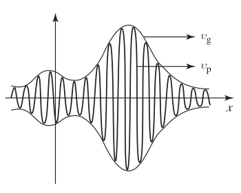
now recalling the stationary state solution form of the full wave function $Ψ = φ ψ$ and from before that $φ \equiv e^{- i E t / ℏ}$ we obtain

Ψ (x, t) = A e^{i k (x - \frac{ℏ k}{2 m} t)} + B e^{- i k (x + \frac{ℏ k}{2 m} t)}

now the first term represents a wave travelling to the right while the second to the left. We denote each term by

Ψ_{k} (x, t) = A e^{i (k x - \frac{ℏ k^{2}}{m} t)}

with $k > 0$ meaning travelling to the right and vice versa for $k < 0$ . Although that by de broglie relation $p = ℏ k$ in quantum the speed of the wave is

v_{quantum} = \frac{ℏ | k |}{2 m} = \sqrt{\frac{E}{2 m}}

which in contrast to the classical speed of free particle with energy E(since $V = 0$ we have $E = (1 / 2) m v^{2}$ i.e pure kinetic) so we have

v_{classical} = \sqrt{\frac{2 E}{m}} = 2 v_{quantum}

so apparently the quantum mechanical wave function travels at half the speed of the particle it is supposed to represent?!

an even bigger problem is that the wave function is not normalizable! just consider

\int_{- \infty}^{\infty} Ψ_{k}^{*} Ψ_{k} d x = | A |^{2} \int_{- \infty}^{\infty} d x = | A |^{2} (\infty)

This means

there is no such thing as free particle with definite energy
the wave solution is not separable for a free particle

Instead if we allow for

a range of $k$ and thus a range of associated energies $p = ℏ k, E = \frac{p^{2}}{2 m}$
the wave function to be a superposition of individually separable solutions for each $k$
Specifically

Ψ (x, t) = \frac{1}{\sqrt{2 π}} \int_{- \infty}^{\infty} ϕ (k) e^{i (k x - \frac{ℏ k^{2}}{2 m} t)} d k

Remark

note although invidually separable, the overall superposition itself is not seperable as you cannot factorize the whole superposition itself $Ψ (x, t)$ into the factors $f (x) g (x)$ . Therefore it remains a fact that the wave solution for a free particle is not separable nor definite. We are only saying that the free particle wave solution admits a "wave packet" solution isntead

then finally unlike before this solution can be normalized for appropriate $ϕ (k)$ .(see this like a special weights that allow for our superpostion to be normalized) We call such a range of energies and speeds a wave packet

Question

now suppose we are given the initial conditions $Ψ (x, 0)$ how do we go about finding $ϕ (k)$ for it?

we use the plancherel theorem(recall Functional Analysis) where we have in our case

ϕ (k) = \frac{1}{\sqrt{2 π}} \int_{- \infty}^{\infty} Ψ (x, 0) e^{- i k x} d x

Now that we have established that finding a separable solution $Ψ_{k} (x, t)$ is not a physical realizable state, we nonetheless still can extract some useful properties. In particle we now consider the group velocity( $v_{g}$ ) of a wave packet instead. By that we don't mean the phase velocity/speed of individual ripples( $v_{p}$ ) each representing the sinusoidal solutions that make up the wave packet but rather the speed of envelop that contains these ripple collectively.

../../../Attachments/Pasted image 20250726004825.png

Theorem

we have

v_{phase} = \frac{ω}{k} and v_{group} = \frac{d ω}{d k}

proof: First start with

Ψ (x, t) = \frac{1}{\sqrt{2 π}} \int_{- \infty}^{+ \infty} ϕ (k) e^{i (k x - ω t)} d k .

where $ω = (ℏ k^{2} / 2 m)$ .then do a taylor expansion

ω (k) \approx ω_{0} + ω_{0}^{'} (k - k_{0})

then do a change of variables from $k$ to $s = k - k_{0}$

Ψ (x, t) \approx \frac{1}{\sqrt{2 π}} \int_{- \infty}^{+ \infty} ϕ (k_{0} + s) e^{i [(k_{0} + s) x - (ω_{0} + ω_{0}^{'} s) t]} d s

= \frac{1}{\sqrt{2 π}} e^{i (k_{0} x - ω_{0} t)} \int_{- \infty}^{+ \infty} ϕ (k_{0} + s) e^{i s (x - ω_{0}^{'} t)} d s .

2.5 The Delta Function Potential

Fact

to summarize so far for the time-independent schrodinger equation we have:

for the infinite square well and harmonic oscillator they are normalizable and labelled by a discrete index n
for the free particle they are non-normalizable and are labnled by the continuous variable k

So you might ask what is the significance of this?
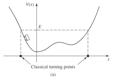
In classical mechanics a one-dimensional time independent can give rise to two different kinds of motion. If $V (x)$ rises higher than the particle's total energy $(E)$ on either side of the (figure a) below, it rocks back for forth between the turning points but it cannot escape. We call this the bound state.

../../../Attachments/Pasted image 20250708234507.png

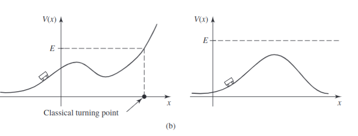
On the other hand $E$ exceeds $V (x)$ on one side or both then the particle comes in from "infinity", slows down or speeds up under the influence of the potential and returns to infinity(figure b). We call this the scattering state

../../../Attachments/Pasted image 20250708234517.png

It turns out that the 2 kinds of solutions to the Schrodinger equation as mentioned above correspond precisely to bound and scattering states. Specifically

{\begin{cases} E < V (- \infty) and V (+ \infty) \Rightarrow bound state, \\ E > V (- \infty) or V (+ \infty) \Rightarrow scattering state. \end{cases}

In real life most potentials go to zero at infinity in which case the criterion simplifies to

{\begin{cases} E < 0 ⟹ bound state, \\ E > 0 ⟹ scattering state. \end{cases}

The Delta Function Well

The dirac delta function is an infinitely high infinitesimally narrow spike at the origin whose area is $1$

δ (x) \equiv {\begin{cases} 0, & if x \neq 0 \\ \infty, & if x = 0 \end{cases}, with \int_{- \infty}^{+ \infty} δ (x) d x = 1.

../../../Attachments/Pasted image 20250708234924.png

Remark

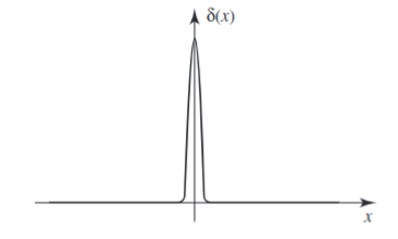
In fact the dirac delta function isn't a function at. The above is just an approximation, in reality the dirac delta function is just a straight line up essentially. Basic high school calculus vertical line test already tells you this can't be a function! More specifically this is a distribution(refer to Distribution Theory and Fourier Analysis for more information)

Let us now consider a potential of the form

V (x) = - α δ (x)

So plugging this into the time independent schrodinger equation we have

- \frac{ℏ^{2}}{2 m} \frac{d^{2} ψ}{d x^{2}} - α δ (x) ψ = E ψ

it yields both bound states( $E < 0$ ) and scattering states( $E > 0$ ). Again we are clearly using the simplification that $V (x) \to 0, x \to \pm \infty$ as with most real life situations. We first consider the case of bound states( $E < 0$ )

In the region $x < 0$ we have $V (x) = 0$ by the definition of delta functions. So

\frac{d^{2}}{d x^{2}} ψ = - \frac{2 m E}{ℏ^{2}} ψ = κ^{2} ψ

where

κ \equiv \frac{\sqrt{- 2 m E}}{ℏ}

since $E < 0$ by assumption $κ \in R^{+}$ so the general solution to the above by basic DE theory is

ψ (x) = A e^{- κ x} + B e^{κ x}

as usual. Now because the first term blows up as $x \to - \infty$ and we must have conservation of probability we must have that $A = 0$ so

ψ (x) = B e^{κ x}, (x < 0)

in the region $x > 0$ where again $V (x) = 0$ this time it is the second term that blows up so

ψ (x) = A e^{- κ x}, (x > 0)

Now we first assume the standard conditions for $ψ$

$ψ$ is always continuous
$d ψ / d x$ is continuous except at points where the potential is infinite
therefore combining the combining the above 2 relations we must have

ψ (x) = {\begin{cases} B e^{κ x} & x \leq 0 \\ B e^{- κ x} & x \geq 0 \end{cases}

which is clearly continuous. Next also see that 2 is indeed satisfied. To see consider the limit $ϵ \to 0$ and integrate the schrodinger equation like so

- \frac{ℏ^{2}}{2 m} \int_{- ϵ}^{+ ϵ} \frac{d^{2} ψ}{d x^{2}} d x + \int_{- ϵ}^{+ ϵ} V (x) ψ (x) d x = E \int_{- ϵ}^{+ ϵ} ψ (x) d x

then we have

Δ (\frac{d ψ}{d x}) \equiv lim_{ϵ \to 0} (\frac{\partial ψ}{\partial x} |_{+ ϵ} - \frac{\partial ψ}{\partial x} |_{- ϵ}) = \frac{2 m}{ℏ^{2}} lim_{ϵ \to 0} \int_{- ϵ}^{+ ϵ} V (x) ψ (x) d x .

since the last integral is zero as $ψ (x)$ is continuous. We know that for $x \neq 0$ we have $V (x) = 0$ by assumption so that we get $Δ (\frac{d ψ}{d x}) = 0$ for all such $x$ as $ϵ \to 0$ . However on the other hand at $x = 0$ we have $V (x) = - α δ (x)$ and so my sifting property we have

Δ (\frac{d ψ}{d x}) = - \frac{2 m α}{ℏ^{2}} ψ (0) = - \frac{2 m α}{ℏ^{2}} B

Remark

from here we also see that the delta function determines the discontinuity in $\frac{d}{d x} ψ$

where from the definition of $ψ$ we know that $ψ (0) = B$ . But at the same time if we differentiate this definition of $ψ$ directly to get $\frac{d}{d x} ψ$ we have

{\begin{cases} d ψ / d x = - B κ e^{- κ x}, for (x > 0), so d ψ / d x |_{+} = - B κ, \\ d ψ / d x = + B κ e^{+ κ x}, for (x < 0), so d ψ / d x |_{-} = + B κ, \end{cases}

therefore we get another expression for the discontinuity $Δ (d ψ / d x) = - 2 B κ$ . Comparing the 2 relations we have for out discontinuity so far we immediately see that

κ = \frac{m α}{ℏ^{2}}

therefore subbing our expressing for $κ$ into previous relation for $κ$ found for bound states we get

E = - \frac{ℏ^{2} κ^{2}}{2 m} = - \frac{m α^{2}}{2 ℏ^{2}}

Question

What is the fourier transform of $δ (x)$ ? Using Planceral's theorem show that

δ (x) = \frac{1}{2 π} \int_{- \infty}^{+ \infty} e^{i k x} d k .

solution: first do as instructed

F {δ (x)} = \frac{1}{\sqrt{2 π}} \int_{- \infty}^{\infty} e^{- i k x} δ (x) d x = \frac{1}{\sqrt{2 π}} e^{- i k (0)} = \frac{1}{\sqrt{2 π}} .

then simply take the inverse fourier transform to get back $δ (x)$ like so

F^{- 1} {F {δ (x)}} = F^{- 1} {\frac{1}{\sqrt{2 π}}}

δ (x) = \frac{1}{\sqrt{2 π}} \int_{- \infty}^{\infty} e^{i k x} (\frac{1}{\sqrt{2 π}}) d k

yielding the result as desired

Question

show that

δ (c x) = \frac{1}{| c |} δ (x)

solution: Consider the integral,

I = \int_{- \infty}^{\infty} f (x) δ (c x) d x .

Assuming that c is positive, make the following substitution.

u = c x \to x = \frac{u}{c}

d u = c d x \to d x = \frac{d u}{c}

Consequently,

I = \int_{c \times - \infty}^{c \times \infty} f (\frac{u}{c}) δ (u) (\frac{d u}{c}) = \frac{1}{c} \int_{- \infty}^{\infty} f (\frac{u}{c}) δ (u) d u = \frac{1}{c} f (0) .

Make the same substitution again, this time assuming that c is negative.

I = \int_{c \times - \infty}^{c \times \infty} f (\frac{u}{c}) δ (u) (\frac{d u}{c}) = \frac{1}{c} \int_{- \infty}^{- \infty} f (\frac{u}{c}) δ (u) d u = - \frac{1}{c} \int_{- \infty}^{\infty} f (\frac{u}{c}) δ (u) d u = - \frac{1}{c} f (0)

Now combine these results.

I = \frac{1}{| c |} f (0) = \frac{1}{| c |} \int_{- \infty}^{\infty} f (x) δ (x) d x = \int_{- \infty}^{\infty} f (x) \frac{δ (x)}{| c |} d x

Therefore,

δ (c x) = \frac{δ (x)}{| c |} .

3. Formalism

3.1 Hilbert Space

Quantum theory is based on two constructs: wave functions and operators. The state of a system is represented by its wave function, observables are represented by operators.

To represent a possible physical state as we know the wave function must be normalized

\int | ψ |^{2} d x = 1

Definition

The set of all square-integrable functions on a specific interval is defined by
$f (x)$ such that $\int_{a}^{b} | f (x) |^{2} d x < \infty$
or basically the $L^{2} (a, b)$ space in the language of mathematicians or the hilbert space in the language of physicts

in particular we are saying that wave functions live in the hilbert space

Definition

The inner product of two functions is written as

⟨ f | g ⟩ \equiv \int_{b}^{a} f (x)^{*} g (x) d x

Remark

this also means that

⟨ a f | f ⟩ = a^{*} ⟨ f | f ⟩ and ⟨ f | a f ⟩ = a ⟨ f | f ⟩

we also have that the inner product with itself

⟨ f | f ⟩ = \int_{a}^{b} | f (x) |^{2} d x

is real and non-negative; it's zero only when $f (x) = 0$ . Refer to Functional Analysis more properties and proofs regarding the inner product.

Definition

The function is said to be normalized if its inner product with itself is 1 and two functions are orthogonal if their inner product is zero and a set of functions ${f_{n}}$ is orthonormal if they are normalized and mutually orthogonal that is

⟨ f_{m} | f_{n} ⟩ = δ_{m n}

Definition

Finally a a set of functions is complete if any other function(in Hilbert space) can be expressed as a linear combination of them

f (x) = \sum_{n = 1}^{\infty} c_{n} f_{n} (x)

If the functions ${f_{n} (x)}$ are orthonormal the cofficients are given by fourier's trick

c_{n} = ⟨ f_{n} | f ⟩

3.2 Observables

3.2.1 Hermitian Operators

Definition

the expectation value of an observa le $Q (x, p)$ can be expressed very neatly in inner-product notation

⟨ Q ⟩ = \int Ψ^{*} \hat{Q} Ψ d x = ⟨ Ψ | \hat{Q} Ψ ⟩

The outcome of a measurement(observable) must be real and so therefore we must have

⟨ Q ⟩ = ⟨ Q^{*} ⟩

For this to happen we must have by definition of expectation value:

⟨ Ψ | \hat{Q} Ψ ⟩ = ⟨ \hat{Q} Ψ | Ψ ⟩

specifically they must have a property where

⟨ f | \hat{Q} f ⟩ = ⟨ \hat{Q} f | f ⟩ for all f (x) .

we call such operators hermitian.

Remark

To emphasize we are essentially saying that observables are represented by hermitian operators(as they must be real)

let us verify this

Example

Consider the momentum operator. Let us check if it is hermitian

⟨ f | \hat{p} g ⟩ = \int_{- \infty}^{\infty} f^{\*} (- i ℏ) \frac{d g}{d x} d x = - i ℏ f^{\*} g |_{- \infty}^{\infty} + \int_{- \infty}^{\infty} {(- i ℏ \frac{d f}{d x})}^{\*} g d x = ⟨ \hat{p} f | g ⟩ .

Definition

The hermitian conjugate(or adjoint) of an operator $\hat{Q}$ is the operator ${\hat{Q}}^{†}$ such that

⟨ f | \hat{Q} g ⟩ = ⟨ {\hat{Q}}^{†} f | g ⟩ (for all f and g) .

note: we are referring to the transpose conjugate specifically hence the above relation

that is a hermitian operator is then equal to its hermitian conjugate $\hat{Q} = {\hat{Q}}^{†}$

Question

Show that if $⟨ h | \hat{Q} h ⟩ = ⟨ \hat{Q} h | h ⟩$ for all h (in Hilbert space), then $⟨ f | \hat{Q} g ⟩ = ⟨ \hat{Q} f | g ⟩$ for all f and g . Hint: First let $h = f + g$ , and then let $h = f + i g$ .

Solution:
Suppose that $⟨ h | Q h ⟩ = ⟨ Q h | h ⟩$ for all h. If $h = f + g$ , then

⟨ h | \hat{Q} h ⟩ = ⟨ h | \hat{Q} | h ⟩ = \int_{a}^{b} h^{\*} (x) \hat{Q} h (x) d x

= \int_{a}^{b} h^{\*} (x) [\hat{Q} h (x)] d x = \int_{a}^{b} [f (x) + g (x)]^{\*} \hat{Q} [f (x) + g (x)] d x

= \int_{a}^{b} [f^{\*} (x) + g^{\*} (x)] [\hat{Q} f (x) + \hat{Q} g (x)] d x = \int_{a}^{b} [f^{\*} (x) \hat{Q} f (x) + f^{\*} (x) \hat{Q} g (x) + g^{\*} (x) \hat{Q} f (x) + g^{\*} (x) \hat{Q} g (x)] d x

= \int_{a}^{b} f^{\*} (x) \hat{Q} f (x) d x + \int_{a}^{b} f^{\*} (x) \hat{Q} g (x) d x + \int_{a}^{b} g^{\*} (x) \hat{Q} f (x) d x + \int_{a}^{b} g^{\*} (x) \hat{Q} g (x) d x

= ⟨ f | \hat{Q} | f ⟩ + ⟨ f | \hat{Q} | g ⟩ + ⟨ g | \hat{Q} | f ⟩ + ⟨ g | \hat{Q} | g ⟩ = ⟨ f | \hat{Q} f ⟩ + ⟨ f | \hat{Q} g ⟩ + ⟨ g | \hat{Q} f ⟩ + ⟨ g | \hat{Q} g ⟩

and

⟨ \hat{Q} h | h ⟩ = ⟨ h | {\hat{Q}}^{†} | h ⟩

= \int_{a}^{b} h^{\*} (x) {\hat{Q}}^{†} h (x) d x = \int_{a}^{b} h^{\*} (x) [{\hat{Q}}^{†} h (x)] d x

= \int_{a}^{b} [f (x) + g (x)]^{\*} {\hat{Q}}^{†} f (x) + g (x) d x

Question

(a) Show that the sum of two hermitian operators is hermitian.
(b) Suppose $\hat{Q}$ is hermitian, and $α$ is a complex number. Under what condition (on $α$ ) is $α \hat{Q}$ hermitian?
(c) When is the product of two hermitian operators hermitian?
(d) Show that the position operator $(\hat{x})$ and the Hamiltonian operator $(\hat{H} = - (ℏ^{2} / 2 m) d^{2} / d x^{2} + V (x))$ are hermitian.

3.2.2 Determinate States

Fact

normally when you measure an observable $Q$ on an ensemble of indentically prepared systems all in the same state $Ψ$ you do not get the same result each time but what if we could get the same value which we denote to be $q$ ? We call such a state a determinate state

Formally this means the variance of $Q$ in a determinate state would be zero which implies

σ^{2} = ⟨ {(Q - ⟨ Q ⟩)}^{2} ⟩ = ⟨ Ψ | {(\hat{Q} - q)}^{2} Ψ ⟩ ⟩ = ⟨ (\hat{Q} - q) Ψ | (\hat{Q} - q) Ψ ⟩ ⟩ = 0.

where we have the final relation because since $Q$ is an observable and thus $\hat{Q}$ is hermitian and that $⟨ Q ⟩ = q \in R$ . Recall these from previously. Also $⟨ Q ⟩ = q$ because obviously the expectation will also be $q$ if every measurement gets $q$ . Finally we recall that by for inner products the only vector in which an inner product with itself yields zero is the zero vector(definiteness of inner product property) and so arrive at

\hat{Q} Ψ = q Ψ

this is basically the eigenvalue equation for the operator $\hat{Q}$ where $Ψ$ is an eigenfunction and $q$ is the eigenvalue.

Fact

To sum up essentially we say that:
Determinate states of Q are eigenfunctions of $\hat{Q}$

Definition

We also say that the collection of all eigenvalues of an operator is called its spectrum and if 2 or more linearly independent eigenfunctions share the same eigenvalue we say such a spectrum is degenerate

3.3 Eigenfunctions of Hermitian Operator

we now turn our attention to eigenfunction of hermitian operators, physically that refers to determinate states of observables if you recall

Theorem

if the spectrum is discrete then the eigenfunctions lie in the Hilbert Space
if the spectrum if continuous then the eigenfunctions are not normalizable

Example

recall the for free particle where we have continuous spectrum, we did not have normalizable eigenfunction unless we considered a "packet". This is in contrast to that of the simple harmonic oscillator which has a discrete spectrum related by ladder operators.

3.3.1 Discrete Spectra

Theorem

their eigenvalues are real

proof suppose

\hat{Q} f = q f

since $\hat{Q}$ is hermitian we have

⟨ f | \hat{Q} f ⟩ = ⟨ \hat{Q} f | f ⟩

then recall first slot of inner product is conjugate linear so

q ⟨ f | f ⟩ = q^{*} ⟨ f | f ⟩

Theorem

the eigenfunctions belonging to distinct eigenvalus are orthogonal

Proof: Suppose

\hat{Q} f = q f, and \hat{Q} g = q^{'} g,

and

\hat{Q} is hermitian. Then ⟨ f | \hat{Q} g ⟩ = ⟨ \hat{Q} f | g ⟩, so

q^{'} ⟨ f | g ⟩ = q^{\*} ⟨ f | g ⟩

(again, the inner products exist because the eigenfunctions are in Hilbert space). But $q$ is real (from Theorem 1), so if $q^{'} e q q$ it must be that $⟨ f | g ⟩ = 0$ . QED

Fact

the eigenfunctions of an observable operator are complete, that is any function in the hilbert space can be expressed as a linear combination of them. This is taken as an axiom in quantum mechanics

more precisely this is done by rtestricting the class of hermitian operators that can represent observables

3.3.2 Continuous Spectra

Question

(a) Cite a Hamiltonian from Chapter 2 (other than the harmonic oscillator) that has only a discrete spectrum.
(b) Cite a Hamiltonian from Chapter 2 (other than the free particle) that has only a continuous spectrum.
(c) Cite a Hamiltonian from Chapter 2 (other than the finite square well) that has both a discrete and a continuous part to its spectrum.

Example

Find the eigenfunctions and eigenvalues of the momentum operator on the interval $- \infty < x < \infty$

solution: Let $f_{p} (x)$ be the eigenfuction and $p$ be the eigenvalue. Then subbing the definition of momentum operator into the eigenvalue equation we get:

- i ℏ \frac{d}{d x} f_{p} (x) = p f_{p} (x)

This is a standard constant coefficient ODE with general solution

f_{p} (x) = A e^{i p x ℏ}

immediately we see this is the same situation as the free particle case(see above). We know this is not normalizable hence the momentum operator has no eigenfunctions in Hilbert space(i.e the square integrable or $L^{2}$ space) as $\int | f_{p} (x) |^{2} d x$ does not converge. Instead we a different kind of normalization. In particular in contrast of above we use different values of $p$ (recall like how we did for wave packets for free particle) and instead of letting $p$ be any complex we restrict it to only real. Specifically we do recalling transform of delta function we have

\int_{- \infty}^{\infty} f_{p^{'}}^{\*} (x) f_{p} (x) d x = | A |^{2} \int_{- \infty}^{\infty} e^{i (p - p^{'}) x / ℏ} d x = | A |^{2} 2 π ℏ δ (p - p^{'}) .

If we pick $A = 1 / \sqrt{2 π h}$ , so that

f_{p} (x) = \frac{1}{\sqrt{2 π h}} e^{i p x / ℏ},

then

⟨ f_{p^{'}} | f_{p} ⟩ = δ (p - p^{'}),

Which is reminisicent of true orthonormality. Basically instead of kronecker delta we have dirac delta. This is known as dirac orthonormality. With this, as usual as physicts we assume that eigenfunctions with real eigenvalues are complete so we have

f (x) = \int_{- \infty}^{\infty} c (p) f_{p} (x) d p = \frac{1}{\sqrt{2 π ℏ}} \int_{- \infty}^{\infty} c (p) e^{i p x / ℏ} d p .

for any square integrable function $f (x)$ . Then the coefficients, i.e the eigenvalues are obtained by plancheral theorem

⟨ f_{p^{'}} | f ⟩ = \int_{- \infty}^{\infty} c (p) ⟨ f_{p^{'}} | f_{p} ⟩ d p = \int_{- \infty}^{\infty} c (p) δ (p - p^{'}) d p = c (p^{'}) .

Question

Similarly find the eigenfunctions and eigenvalues of the position operator

solution: Let $g_{y} (x)$ be the eigenfunction and y the eigenvalue:

\hat{x} g_{y} (x) = x g_{y} (x) = y g_{y} (x) .

see that $y$ is a fixed number(the eigenvalue) while $x$ is a continuous variable. It is that immediately clear that we must have $g_{y} = 0$ only except when $x = y$ . That precisely defines the delta function.

g_{y} (x) = A δ (x - y)

just like above we then know that such eigenfunction are not square integrable but rather are Dirac orthonormal

3.4 Generalized statistical Interpretation

Quick recap basics first. Recall that eigenfunctions of an observable operator are complete that is

Ψ (x, t) = \sum_{n} c_{n} (t) f_{n} (x) .

and because the eigenfunctions are orthonormal we have

c_{n} (t) = ⟨ f_{n} | Ψ ⟩ = \int f_{n} (x)^{\*} Ψ (x, t) d x .

Proposition

$\sum_{n} | c_{n} |^{2} = 1$

proof consider

1 = ⟨ Ψ | Ψ ⟩ = ⟨ (\sum_{n^{'}} c_{n^{'}} f_{n^{'}}) | (\sum_{n} c_{n} f_{n}) ⟩ = \sum_{n^{'}} \sum_{n^{'}} c_{n^{'}}^{\*} c_{n} ⟨ f_{n^{'}} | f_{n} ⟩

= \sum_{n^{'}} \sum_{n} c_{n^{'}}^{\*} c_{n} δ_{n^{'} n} = \sum_{n} c_{n}^{\*} c_{n} = \sum_{n} | c_{n} |^{2} .

where recall from the start that we must have $\int_{- \infty}^{+ \infty} | Ψ (x, t) |^{2} d x = 1.$ .

Proposition

Similarly we have

⟨ Q ⟩ = \sum_{n} q_{n} | c_{n} |^{2}

proof: Consider

⟨ Q ⟩ = ⟨ Ψ | \hat{Q} Ψ ⟩ = ⟨ (\sum_{n^{'}} c_{n^{'}} f_{n^{'}}) | (\hat{Q} \sum_{n} c_{n} f_{n}) ⟩,

but $\hat{Q} f_{n} = q_{n} f_{n}$ , so

⟨ Q ⟩ = \sum_{n^{'}} \sum_{n} c_{n}^{\*} c_{n} q_{n} ⟨ f_{n^{'}} | f_{n} ⟩ = \sum_{n^{'}} \sum_{n^{'}} c_{n^{'}}^{\*} c_{n} q_{n} δ_{n^{'} n} = \sum_{n} q_{n} | c_{n} |^{2} .